Let’s face it, robots are cool. They’re also going to run the world some day, and hopefully, at that time they will take pity on their poor soft fleshy creators (a.k.a. robotics developers) and help us build a space utopia filled with plenty. I’m joking of course, but only sort of.

In my ambition to have some small influence over the matter, I took a course in autonomous robot control theory last year, which culminated in my building a Python-based robotic simulator that allowed me to practice control theory on a simple, mobile, programmable robot.
Video
In this article, I’m going to show how to use a Python robot framework to develop control software, describe the control scheme I developed for my simulated robot, illustrate how it interacts with its environment and achieves its goals, and discuss some of the fundamental challenges of robotics programming that I encountered along the way.
In order to follow this tutorial on robotics programming for beginners, you should have a basic knowledge of two things:
Mathematics—we will use some trigonometric functions and vectors
Python—since Python is among the more popular basic robot programming languages—we will make use of basic Python libraries and functions
The snippets of code shown here are just a part of the entire simulator, which relies on classes and interfaces, so in order to read the code directly, you may need some experience in Python and object oriented programming.
Finally, optional topics that will help you to better follow this tutorial are knowing what a state machine is and how range sensors and encoders work.
The challenge of the programmable robot: perception versus reality, and the fragility of control
The fundamental challenge of all robotics is this: It is impossible to ever know the true state of the environment. Robot control software can only guess the state of the real world based on measurements returned by its sensors. It can only attempt to change the state of the real world through the generation of control signals.
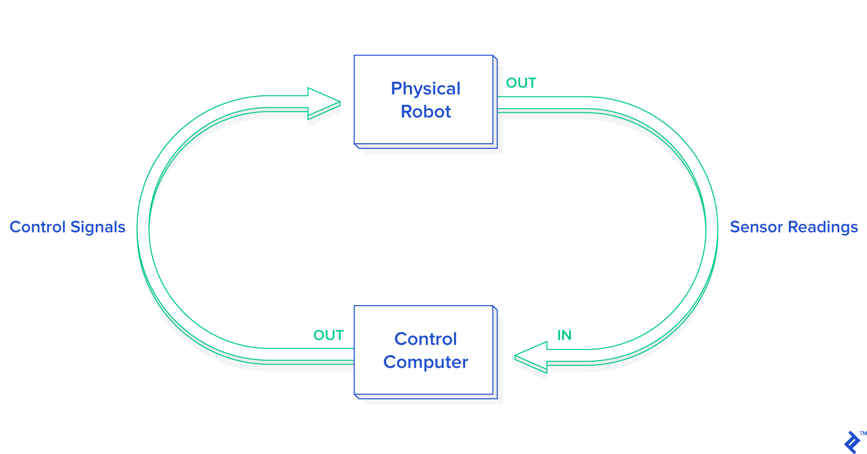
Thus, one of the first steps in control design is to come up with an abstraction of the real world, known as a model, with which to interpret our sensor readings and make decisions. As long as the real world behaves according to the assumptions of the model, we can make good guesses and exert control. As soon as the real world deviates from these assumptions, however, we will no longer be able to make good guesses, and control will be lost. Often, once control is lost, it can never be regained. (Unless some benevolent outside force restores it.)
This is one of the key reasons that robotics programming is so difficult. We often see videos of the latest research robot in the lab, performing fantastic feats of dexterity, navigation, or teamwork, and we are tempted to ask, “Why isn’t this used in the real world?” Well, next time you see such a video, take a look at how highly-controlled the lab environment is. In most cases, these robots are only able to perform these impressive tasks as long as the environmental conditions remain within the narrow confines of its internal model. Thus, one key to the advancement of robotics is the development of more complex, flexible, and robust models—and said advancement is subject to the limits of the available computational resources.
One key to the advancement of robotics is the development of more complex, flexible, and robust models.
[Side Note: Philosophers and psychologists alike would note that living creatures also suffer from dependence on their own internal perception of what their senses are telling them. Many advances in robotics come from observing living creatures and seeing how they react to unexpected stimuli. Think about it. What is your internal model of the world? It is different from that of an ant, and that of a fish? (Hopefully.) However, like the ant and the fish, it is likely to oversimplify some realities of the world. When your assumptions about the world are not correct, it can put you at risk of losing control of things. Sometimes we call this “danger.” The same way our little robot struggles to survive against the unknown universe, so do we all. This is a powerful insight for roboticists.]
The programmable robot simulator
The simulator I built is written in Python and very cleverly dubbed Sobot Rimulator. You can find v1.0.0 on GitHub. It does not have a lot of bells and whistles but it is built to do one thing very well: provide an accurate simulation of a mobile robot and give an aspiring roboticist a simple framework for practicing robot software programming. While it is always better to have a real robot to play with, a good Python robot simulator is much more accessible and is a great place to start.
In real-world robots, the software that generates the control signals (the “controller”) is required to run at a very high speed and make complex computations. This affects the choice of which robot programming languages are best to use: Usually, C++ is used for these kinds of scenarios, but in simpler robotics applications, Python is a very good compromise between execution speed and ease of development and testing.
The software I wrote simulates a real-life research robot called the Khepera but it can be adapted to a range of mobile robots with different dimensions and sensors. Since I tried to program the simulator as similar as possible to the real robot’s capabilities, the control logic can be loaded into a real Khepera robot with minimal refactoring, and it will perform the same as the simulated robot. The specific features implemented refer to the Khepera III, but they can be easily adapted to the new Khepera IV.
In other words, programming a simulated robot is analogous to programming a real robot. This is critical if the simulator is to be of any use to develop and evaluate different control software approaches.
In this tutorial, I will be describing the robot control software architecture that comes with v1.0.0 of Sobot Rimulator, and providing snippets from the Python source (with slight modifications for clarity). However, I encourage you to dive into the source and mess around. The simulator has been forked and used to control different mobile robots, including a Roomba2 from iRobot. Likewise, please feel free to fork the project and improve it.
The control logic of the robot is constrained to these Python classes/files:
models/supervisor.py—this class is responsible for the interaction between the simulated world around the robot and the robot itself. It evolves our robot state machine and triggers the controllers for computing the desired behavior.
models/supervisor_state_machine.py—this class represents the different states in which the robot can be, depending on its interpretation of the sensors.
The files in the models/controllers directory—these classes implement different behaviors of the robot given a known state of the environment. In particular, a specific controller is selected depending on the state machine.
The goal
Robots, like people, need a purpose in life. The goal of our software controlling this robot will be very simple: It will attempt to make its way to a predetermined goal point. This is usually the basic feature that any mobile robot should have, from autonomous cars to robotic vacuum cleaners. The coordinates of the goal are programmed into the control software before the robot is activated but could be generated from an additional Python application that oversees the robot movements. For example, think of it driving through multiple waypoints.
However, to complicate matters, the environment of the robot may be strewn with obstacles. The robot MAY NOT collide with an obstacle on its way to the goal. Therefore, if the robot encounters an obstacle, it will have to find its way around so that it can continue on its way to the goal.
The programmable robot
Every robot comes with different capabilities and control concerns. Let’s get familiar with our simulated programmable robot.
The first thing to note is that, in this guide, our robot will be an autonomous mobile robot. This means that it will move around in space freely and that it will do so under its own control. This is in contrast to, say, a remote-control robot (which is not autonomous) or a factory robot arm (which is not mobile). Our robot must figure out for itself how to achieve its goals and survive in its environment. This proves to be a surprisingly difficult challenge for novice robotics programmers.
Control inputs: sensors
There are many different ways a robot may be equipped to monitor its environment. These can include anything from proximity sensors, light sensors, bumpers, cameras, and so forth. In addition, robots may communicate with external sensors that give them information that they themselves cannot directly observe.
Our reference robot is equipped with nine infrared sensors—the newer model has eight infrared and five ultrasonic proximity sensors—arranged in a “skirt” in every direction. There are more sensors facing the front of the robot than the back because it is usually more important for the robot to know what is in front of it than what is behind it.
In addition to the proximity sensors, the robot has a pair of wheel tickers that track wheel movement. These allow you to track how many rotations each wheel makes, with one full forward turn of a wheel being 2,765 ticks. Turns in the opposite direction count backward, decreasing the tick count instead of increasing it. You don’t have to worry about specific numbers in this tutorial because the software we will write uses the traveled distance expressed in meters. Later I will show you how to compute it from ticks with an easy Python function.
Control Outputs: mobility
Some robots move around on legs. Some roll like a ball. Some even slither like a snake.
Our robot is a differential drive robot, meaning that it rolls around on two wheels. When both wheels turn at the same speed, the robot moves in a straight line. When the wheels move at different speeds, the robot turns. Thus, controlling the movement of this robot comes down to properly controlling the rates at which each of these two wheels turn.
API
In Sobot Rimulator, the separation between the robot “computer” and the (simulated) physical world is embodied by the file robot_supervisor_interface.py, which defines the entire API for interacting with the “real robot” sensors and motors:
read_proximity_sensors() returns an array of nine values in the sensors’ native format
read_wheel_encoders() returns an array of two values indicating total ticks since the start
set_wheel_drive_rates( v_l, v_r ) takes two values (in radians-per-second) and sets the left and right speed of the wheels to those two values
This interface internally uses a robot object that provides the data from sensors and the possibility to move motors or wheels. If you want to create a different robot, you simply have to provide a different Python robot class that can be used by the same interface, and the rest of the code (controllers, supervisor, and simulator) will work out of the box!
The simulator
As you would use a real robot in the real world without paying too much attention to the laws of physics involved, you can ignore how the robot is simulated and just skip directly to how the controller software is programmed, since it will be almost the same between the real world and a simulation. But if you are curious, I will briefly introduce it here.
The file world.py is a Python class that represents the simulated world, with robots and obstacles inside. The step function inside this class takes care of evolving our simple world by:
Applying physics rules to the robot’s movements
Considering collisions with obstacles
Providing new values for the robot sensors
In the end, it calls the robot supervisors responsible for executing the robot brain software.
The step function is executed in a loop so that robot.step_motion() moves the robot using the wheel speed computed by the supervisor in the previous simulation step.
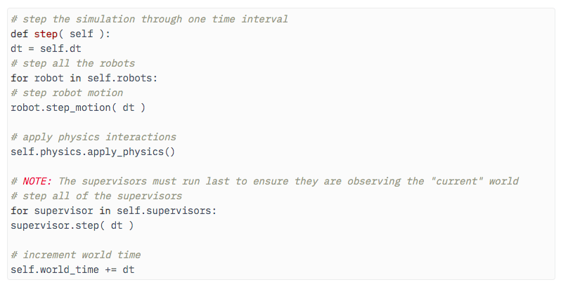
The apply_physics() function internally updates the values of the robot proximity sensors so that the supervisor will be able to estimate the environment at the current simulation step. The same concepts apply to the encoders.
A simple model
First, our robot will have a very simple model. It will make many assumptions about the world. Some of the important ones include:
The terrain is always flat and even
Obstacles are never round
The wheels never slip
Nothing is ever going to push the robot around
The sensors never fail or give false readings
The wheels always turn when they are told to
Although most of these assumptions are reasonable inside a house-like environment, round obstacles could be present. Our obstacle avoidance software has a simple implementation and follows the border of obstacles in order to go around them. We will hint readers on how to improve the control framework of our robot with an additional check to avoid circular obstacles.
The control loop
We will now enter into the core of our control software and explain the behaviors that we want to program inside the robot. Additional behaviors can be added to this framework, and you should try your own ideas after you finish reading! Behavior-based robotics software was proposed more than 20 years ago and it’s still a powerful tool for mobile robotics. As an example, in 2007 a set of behaviors was used in the DARPA Urban Challenge—the first competition for autonomous driving cars!
A robot is a dynamic system. The state of the robot, the readings of its sensors, and the effects of its control signals are in constant flux. Controlling the way events play out involves the following three steps:
Apply control signals.
Measure the results.
Generate new control signals calculated to bring us closer to our goal.
These steps are repeated over and over until we have achieved our goal. The more times we can do this per second, the finer control we will have over the system. The Sobot Rimulator robot repeats these steps 20 times per second (20 Hz), but many robots must do this thousands or millions of times per second in order to have adequate control. Remember our previous introduction about different robot programming languages for different robotics systems and speed requirements.
In general, each time our robot takes measurements with its sensors, it uses these measurements to update its internal estimate of the state of the world—for example, the distance from its goal. It compares this state to a reference value of what it wants the state to be (for the distance, it wants it to be zero), and calculates the error between the desired state and the actual state. Once this information is known, generating new control signals can be reduced to a problem of minimizing the error which will eventually move the robot towards the goal.
A nifty trick: simplifying the model
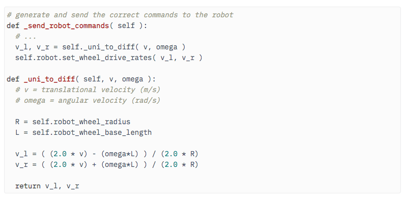
To control the robot we want to program, we have to send a signal to the left wheel telling it how fast to turn, and a separate signal to the right wheel telling it how fast to turn. Let’s call these signals vL and vR. However, constantly thinking in terms of vL and vR is very cumbersome. Instead of asking, “How fast do we want the left wheel to turn, and how fast do we want the right wheel to turn?” it is more natural to ask, “How fast do we want the robot to move forward, and how fast do we want it to turn, or change its heading?” Let’s call these parameters velocity v and angular (rotational) velocity ω (read “omega”). It turns out we can base our entire model on v and ω instead of vL and vR, and only once we have determined how we want our programmed robot to move, mathematically transform these two values into the vL and vR we need to actually control the robot wheels. This is known as a unicycle model of control.
Here is the Python code that implements the final transformation in supervisor.py. Note that if ω is 0, both wheels will turn at the same speed:
Estimating state: robot, know thyself
Using its sensors, the robot must try to estimate the state of the environment as well as its own state. These estimates will never be perfect, but they must be fairly good because the robot will be basing all of its decisions on these estimations. Using its proximity sensors and wheel tickers alone, it must try to guess the following:
The direction to obstacles
The distance from obstacles
The position of the robot
The heading of the robot
The first two properties are determined by the proximity sensor readings and are fairly straightforward. The API function read_proximity_sensors() returns an array of nine values, one for each sensor. We know ahead of time that the seventh reading, for example, corresponds to the sensor that points 75 degrees to the right of the robot.
Thus, if this value shows a reading corresponding to 0.1 meters distance, we know that there is an obstacle 0.1 meters away, 75 degrees to the left. If there is no obstacle, the sensor will return a reading of its maximum range of 0.2 meters. Thus, if we read 0.2 meters on sensor seven, we will assume that there is actually no obstacle in that direction.
Because of the way the infrared sensors work (measuring infrared reflection), the numbers they return are a non-linear transformation of the actual distance detected. Thus, the Python function for determining the distance indicated must convert these readings into meters. This is done in supervisor.py as follows:

Again, we have a specific sensor model in this Python robot framework, while in the real world, sensors come with accompanying software that should provide similar conversion functions from non-linear values to meters.
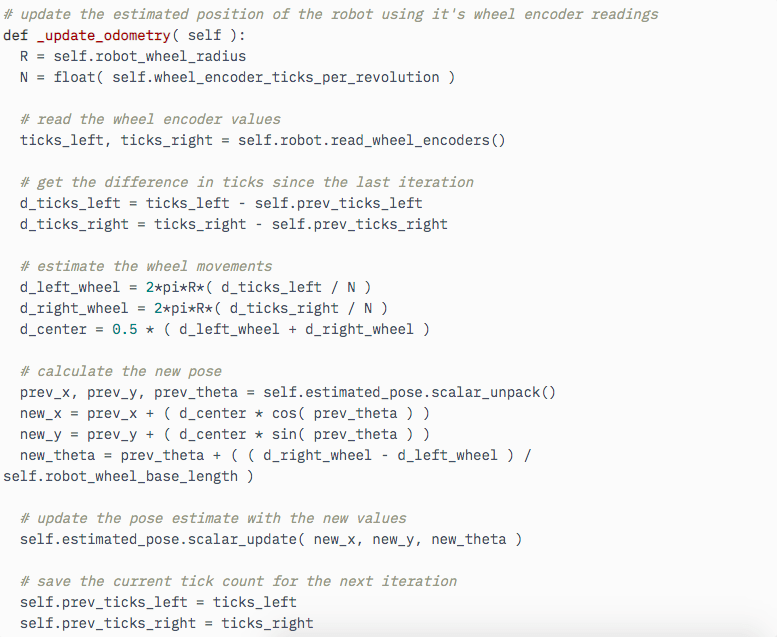
Determining the position and heading of the robot (together known as the pose in robotics programming) is somewhat more challenging. Our robot uses odometry to estimate its pose. This is where the wheel tickers come in. By measuring how much each wheel has turned since the last iteration of the control loop, it is possible to get a good estimate of how the robot’s pose has changed—but only if the change is small.
This is one reason it is important to iterate the control loop very frequently in a real-world robot, where the motors moving the wheels may not be perfect. If we waited too long to measure the wheel tickers, both wheels could have done quite a lot, and it will be impossible to estimate where we have ended up.
Given our current software simulator, we can afford to run the odometry computation at 20 Hz—the same frequency as the controllers. But it could be a good idea to have a separate Python thread running faster to catch smaller movements of the tickers.
Below is the full odometry function in supervisor.py that updates the robot pose estimation. Note that the robot’s pose is composed of the coordinates x and y, and the heading theta, which is measured in radians from the positive X-axis. Positive x is to the east and positive y is to the north. Thus a heading of 0 indicates that the robot is facing directly east. The robot always assumes its initial pose is (0, 0), 0.
Now that our robot is able to generate a good estimate of the real world, let’s use this information to achieve our goals.
Python robot programming methods: go-to-Goal behavior
The supreme purpose in our little robot’s existence in this programming tutorial is to get to the goal point. So how do we make the wheels turn to get it there? Let’s start by simplifying our worldview a little and assume there are no obstacles in the way.
This then becomes a simple task and can be easily programmed in Python. If we go forward while facing the goal, we will get there. Thanks to our odometry, we know what our current coordinates and heading are. We also know what the coordinates of the goal are because they were pre-programmed. Therefore, using a little linear algebra, we can determine the vector from our location to the goal, as in go_to_goal_controller.py:

Note that we are getting the vector to the goal in the robot’s reference frame, and NOT in world coordinates. If the goal is on the X-axis in the robot’s reference frame, that means it is directly in front of the robot. Thus, the angle of this vector from the X-axis is the difference between our heading and the heading we want to be on. In other words, it is the error between our current state and what we want our current state to be. We, therefore, want to adjust our turning rate ω so that the angle between our heading and the goal will change towards 0. We want to minimize the error:

self.kP in the above snippet of the controller Python implementation is a control gain. It is a coefficient which determines how fast we turn in proportion to how far away from the goal we are facing. If the error in our heading is 0, then the turning rate is also 0. In the real Python function inside the file go_to_goal_controller.py, you will see more similar gains, since we used a PID controller instead of a simple proportional coefficient.
Now that we have our angular velocity ω, how do we determine our forward velocity v? A good general rule of thumb is one you probably know instinctively: If we are not making a turn, we can go forward at full speed, and then the faster we are turning, the more we should slow down. This generally helps us keep our system stable and acting within the bounds of our model. Thus, v is a function of ω. In go_to_goal_controller.py the equation is:

A suggestion to elaborate on this formula is to consider that we usually slow down when near the goal in order to reach it with zero speed. How would this formula change? It has to include somehow a replacement of v_max() with something proportional to the distance. OK, we have almost completed a single control loop. The only thing left to do is transform these two unicycle-model parameters into differential wheel speeds, and send the signals to the wheels. Here’s an example of the robot’s trajectory under the go-to-goal controller, with no obstacles:
As we can see, the vector to the goal is an effective reference for us to base our control calculations on. It is an internal representation of “where we want to go.” As we will see, the only major difference between go-to-goal and other behaviors is that sometimes going towards the goal is a bad idea, so we must calculate a different reference vector.
Python robot programming methods: avoid-obstacles behavior
Going towards the goal when there’s an obstacle in that direction is a case in point. Instead of running headlong into things in our way, let’s try to program a control law that makes the robot avoid them.
To simplify the scenario, let’s now forget the goal point completely and just make the following our objective: When there are no obstacles in front of us, move forward. When an obstacle is encountered, turn away from it until it is no longer in front of us.
Accordingly, when there is no obstacle in front of us, we want our reference vector to simply point forward. Then ω will be zero and v will be maximum speed. However, as soon as we detect an obstacle with our proximity sensors, we want the reference vector to point in whatever direction is away from the obstacle. This will cause ω to shoot up to turn us away from the obstacle, and cause v to drop to make sure we don’t accidentally run into the obstacle in the process.
A neat way to generate our desired reference vector is by turning our nine proximity readings into vectors, and taking a weighted sum. When there are no obstacles detected, the vectors will sum symmetrically, resulting in a reference vector that points straight ahead as desired. But if a sensor on, say, the right side picks up an obstacle, it will contribute a smaller vector to the sum, and the result will be a reference vector that is shifted towards the left.
For a general robot with a different placement of sensors, the same idea can be applied but may require changes in the weights and/or additional care when sensors are symmetrical in front and in the rear of the robot, as the weighted sum could become zero.
Here is the code that does this in avoid_obstacles_controller.py:
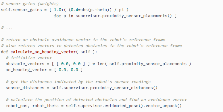
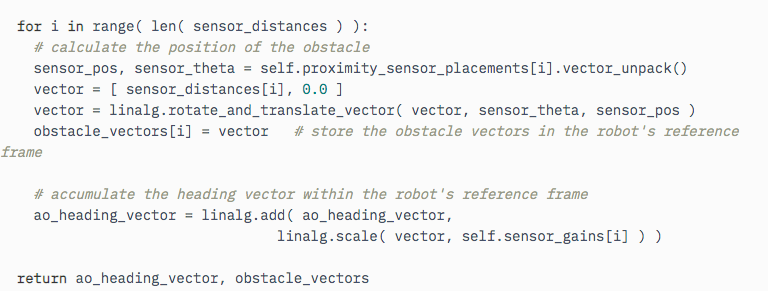
Using the resulting ao_heading_vector as our reference for the robot to try to match, here are the results of running the robot software in simulation using only the avoid-obstacles controller, ignoring the goal point completely. The robot bounces around aimlessly, but it never collides with an obstacle, and even manages to navigate some very tight spaces:
Python robot programming methods: hybrid automata (behavior state machine)
So far we’ve described two behaviors—go-to-goal and avoid-obstacles—in isolation. Both perform their function admirably, but in order to successfully reach the goal in an environment full of obstacles, we need to combine them.
The solution we will develop lies in a class of machines that has the supremely cool-sounding designation of hybrid automata. A hybrid automaton is programmed with several different behaviors, or modes, as well as a supervising state machine. The supervising state machine switches from one mode to another in discrete times (when goals are achieved or the environment suddenly changed too much), while each behavior uses sensors and wheels to react continuously to environment changes. The solution was called hybrid because it evolves both in a discrete and continuous fashion.
Our Python robot framework implements the state machine in the file supervisor_state_machine.py.
Equipped with our two handy behaviors, a simple logic suggests itself: When there is no obstacle detected, use the go-to-goal behavior. When an obstacle is detected, switch to the avoid-obstacles behavior until the obstacle is no longer detected.
As it turns out, however, this logic will produce a lot of problems. What this system will tend to do when it encounters an obstacle is to turn away from it, then as soon as it has moved away from it, turn right back around and run into it again. The result is an endless loop of rapid switching that renders the robot useless. In the worst case, the robot may switch between behaviors with every iteration of the control loop—a state known as a Zeno condition.
There are multiple solutions to this problem, and readers that are looking for deeper knowledge should check, for example, the DAMN software architecture.
What we need for our simple simulated robot is an easier solution: One more behavior specialized with the task of getting around an obstacle and reaching the other side.
Python robot programming methods: follow-wall behavior
Here’s the idea: When we encounter an obstacle, take the two sensor readings that are closest to the obstacle and use them to estimate the surface of the obstacle. Then, simply set our reference vector to be parallel to this surface. Keep following this wall until A) the obstacle is no longer between us and the goal, and B) we are closer to the goal than we were when we started. Then we can be certain we have navigated the obstacle properly.
With our limited information, we can’t say for certain whether it will be faster to go around the obstacle to the left or to the right. To make up our minds, we select the direction that will move us closer to the goal immediately. To figure out which way that is, we need to know the reference vectors of the go-to-goal behavior and the avoid-obstacle behavior, as well as both of the possible follow-wall reference vectors. Here is an illustration of how the final decision is made (in this case, the robot will choose to go left):
Determining the follow-wall reference vectors turns out to be a bit more involved than either the avoid-obstacle or go-to-goal reference vectors. Take a look at the Python code in follow_wall_controller.py to see how it’s done.
Final control design
The final control design uses the follow-wall behavior for almost all encounters with obstacles. However, if the robot finds itself in a tight spot, dangerously close to a collision, it will switch to pure avoid-obstacles mode until it is a safer distance away, and then return to follow-wall. Once obstacles have been successfully negotiated, the robot switches to go-to-goal. Here is the final state diagram, which is programmed inside the supervisor_state_machine.py:
Here is the robot successfully navigating a crowded environment using this control scheme:
An additional feature of the state machine that you can try to implement is a way to avoid circular obstacles by switching to go-to-goal as soon as possible instead of following the obstacle border until the end (which does not exist for circular objects!)
Tweak, tweak, tweak: trial and error
The control scheme that comes with Sobot Rimulator is very finely tuned. It took many hours of tweaking one little variable here, and another equation there, to get it to work in a way I was satisfied with. Robotics programming often involves a great deal of plain old trial-and-error. Robots are very complex and there are few shortcuts to getting them to behave optimally in a robot simulator environment…at least, not much short of outright machine learning, but that’s a whole other can of worms.
Robotics often involves a great deal of plain old trial-and-error.
I encourage you to play with the control variables in Sobot Rimulator and observe and attempt to interpret the results. Changes to the following all have profound effects on the simulated robot’s behavior:
The error gain kP in each controller
The sensor gains used by the avoid-obstacles controller
The calculation of v as a function of ω in each controller
The obstacle standoff distance used by the follow-wall controller
The switching conditions used by supervisor_state_machine.py
Pretty much anything else
When programmable robots fail
We’ve done a lot of work to get to this point, and this robot seems pretty clever. Yet, if you run Sobot Rimulator through several randomized maps, it won’t be long before you find one that this robot can’t deal with. Sometimes it drives itself directly into tight corners and collides. Sometimes it just oscillates back and forth endlessly on the wrong side of an obstacle. Occasionally it is legitimately imprisoned with no possible path to the goal. After all of our testing and tweaking, sometimes we must come to the conclusion that the model we are working with just isn’t up to the job, and we have to change the design or add functionality.
In the mobile robot universe, our little robot’s “brain” is on the simpler end of the spectrum. Many of the failure cases it encounters could be overcome by adding some more advanced software to the mix. More advanced robots make use of techniques such as mapping, to remember where it’s been and avoid trying the same things over and over; heuristics, to generate acceptable decisions when there is no perfect decision to be found; and machine learning, to more perfectly tune the various control parameters governing the robot’s behavior.
A sample of what’s to come
Robots are already doing so much for us, and they are only going to be doing more in the future. While even basic robotics programming is a tough field of study requiring great patience, it is also a fascinating and immensely rewarding one.
In this tutorial, we learned how to develop reactive control software for a robot using the high-level programming language Python. But there are many more advanced concepts that can be learned and tested quickly with a Python robot framework similar to the one we prototyped here. I hope you will consider getting involved in the shaping of things to come.
A beginner’s guide to robot programming with Python
 Reviewed by Tejkiran Kushwaha
on
July 12, 2020
Rating:
 Reviewed by Tejkiran Kushwaha
on
July 12, 2020
Rating:

I definitely enjoying every little bit of it. It is a great website and nice share. I want to thank you. Good job! You guys do a great blog, and have some great contents. Keep up the good work. hitechwork
ReplyDelete